%PL - some issues/questions

Paul - thanks!

I implemented it and now it works as I want.

Martin,

Take a look at this.

module example
implicit none
integer, parameter :: dp = kind(1.d0), n = 1000
real(kind=dp), parameter :: pi = 3.14159265359d0, dt = 1.d-4, omega = 50.d0*2.d0*pi, ta = 0.040d0
real(kind=dp) t1(1:n), ac(1:n), dc(1:n), inst(1:n), xmin_data, xmax_data, ymin_data, ymax_data, xstep, ystep
real(kind=dp) x_min_now, x_max_now, y_min_now, y_max_now
contains
  integer function generate_data()
  integer i
    do i = 1, n, 1
      if (i .gt. 1) then
        t1(i) = t1(i-1) + dt
      else
        t1(i) = 0.d0
      end if
      ac(i) = sqrt(2.d0)*cos(omega*t1(i)-pi)  ;  dc(i) = -ac(1)*exp(-t1(i)/ta) ; inst(i)=ac(i)+dc(i)
    end do
    generate_data = 1
  end function generate_data

  integer function plot()
  include<windows.ins>
  integer, save :: iw
    xmin_data = minval(t1)  ; xmax_data = maxval(t1) 
    ymin_data = min(minval(ac), minval(dc), minval(inst)) ; ymax_data = max(maxval(ac), maxval(dc), maxval(inst))
    xstep = (xmax_data - xmin_data)/10.d0 ; ystep = (ymax_data - ymin_data)/10.d0
    x_min_now = xmin_data ; x_max_now = xmax_data ; y_min_now = ymin_data ; y_max_now = ymax_data
    call winop@('%pl[native,x_array,gridlines,n_graphs=3,width=2,frame,etched,colour=blue,colour=red,colour=black]')
    iw = winio@('%pl[full_mouse_input]&',700,600,n,t1,ac,dc,inst)
    iw = winio@('%ob[scored]&')
    iw = winio@('%2nl%cn%^tt[Zoom in]&',              zoom_in_cb)
    iw = winio@('%2nl%cn%^tt[Zoom out]&',             zoom_out_cb)
    iw = winio@('%2nl%cn%^tt[Full extents]%2nl&',     zoom_out_full_cb)
    iw = winio@('%2nl%cn%^tt[Pan pos X]&',            pan_positive_x_cb)
    iw = winio@('%2nl%cn%^tt[Pan neg X]&',            pan_negative_x_cb)
    iw = winio@('%2nl%cn%^tt[Pan pos Y]&',            pan_positive_y_cb)
    iw = winio@('%2nl%cn%^tt[Pan neg Y]&',            pan_negative_y_cb)
    iw = winio@('%cb%ff%2nl%cn%tt[Close]&')
    iw = winio@(' ') ; plot = 1
  end function plot


  integer function update_pl_limits()
  include<windows.ins>
  integer k
    k = CHANGE_PLOT_DBL@(0, 'x_min', 0, x_min_now) ; k = CHANGE_PLOT_DBL@(0, 'x_max', 0, x_max_now)
    k = CHANGE_PLOT_DBL@(0, 'y_min', 0, y_min_now) ; k = CHANGE_PLOT_DBL@(0, 'y_max', 0, y_max_now)
    call simpleplot_redraw@()           
    update_pl_limits = 1
  end function update_pl_limits


  subroutine swap_real_dp(r1,r2)
  real(kind=dp), intent(inout) :: r1, r2
  real(kind=dp) temp
    temp = r2 ; r2 = r1 ; r1 = temp
  end subroutine swap_real_dp
  

  integer function zoom_out_cb()
  include<windows.ins>
  integer i
    x_min_now = x_min_now - xstep ; x_max_now = x_max_now + xstep ; y_min_now = y_min_now - ystep ; y_max_now = y_max_now + ystep
    i = update_pl_limits() ; zoom_out_cb = 1
  end function zoom_out_cb

[/quote]

Part 2

  integer function zoom_in_cb()
  real(kind=dp) x_min_now_save, x_max_now_save, y_min_now_save, y_max_now_save
  integer i
  integer, save :: iw
    x_min_now_save = x_min_now ; x_max_now_save = x_max_now  ; y_min_now_save = y_min_now ; y_max_now_save = y_max_now
    x_min_now = x_min_now + xstep ; x_max_now = x_max_now - xstep ; y_min_now = y_min_now + ystep ; y_max_now = y_max_now - ystep
    if ( ( x_max_now - x_min_now .gt. xstep ) .and. ( y_max_now - y_min_now .gt. xstep ) ) then
      i = update_pl_limits()
    else
      x_min_now = x_min_now_save ; x_max_now = x_max_now_save ; y_min_now = y_min_now_save ; y_max_now = y_max_now_save
      iw = winio@('%ws%2nl%cn%tt[Continue]','Max zoom level with this control.')  
    end if
   zoom_in_cb = 1
  end function zoom_in_cb


  integer function zoom_out_full_cb()
  integer i
    x_min_now = xmin_data ; y_min_now = ymin_data ; x_max_now = xmax_data ; y_max_now = ymax_data ; i = update_pl_limits()
    zoom_out_full_cb = 1
  end function zoom_out_full_cb


  integer function pan_positive_x_cb()
  integer i
    x_min_now = x_min_now + xstep ; x_max_now = x_max_now + xstep ; i = update_pl_limits() ; pan_positive_x_cb = 1
  end function pan_positive_x_cb


  integer function pan_negative_x_cb()
  integer i
    x_min_now = x_min_now - xstep ; x_max_now = x_max_now - xstep ; i = update_pl_limits() ; pan_negative_x_cb = 1
  end function pan_negative_x_cb


  integer function pan_positive_y_cb()
  integer i
    y_min_now = y_min_now + ystep ; y_max_now = y_max_now + ystep ; i = update_pl_limits() ; pan_positive_y_cb = 1
  end function pan_positive_y_cb  

  
  integer function pan_negative_y_cb()
  integer i
    y_min_now = y_min_now - ystep ; y_max_now = y_max_now - ystep ; i = update_pl_limits() ; pan_negative_y_cb = 1
  end function pan_negative_y_cb 


end module example 

program main
use example
implicit none
integer i
i = generate_data() ; i = plot()
end program main

Ken - huge thanks!

I will review your code thoroughly and will try to implement it. Just one thing is not quite clear for me at the moment (after first review of your code).

One line of your code says:

   iw = winio@('%pl[full_mouse_input]&',700,600,n,t1,ac,dc,inst)

Are the INST values for the 4th graphs? (you specified in the preceding statement that N_GRAPHS=3 and in the code above seems to me that the 4th argument INST should provide the values for the 4th graph. When you specified N_GRAPHS=3, why do you use 4 arguments: t1 array, ac array, dc array and inst array? There should be only 3 arguments - t1,ac,dc. Am I wrong with this interpretation?).

Martin

Martin,

In this case I am not using the [independent] option. There are three graphs to be plotted. ac vs. t1 i.e. Y1 vs X (a sinusoidal wave) dc vs. tt i.e. Y2 vs X (a decaying dc wave) inst vs. t1 i.e. Y3 vs X (the sum of these waves – at this point you may realise I am an electrical engineer).

Looking again at the code, in this case you can dispense with the [full_mouse_input] option. That’s a hangover from something that did not work as I expected it to with certain combinations of compiler options. For the same reason you can delete the subroutine swap_real_dp.

So the call to %pl should be:

call winop@('%pl[native,x_array,gridlines,n_graphs=3,width=2,frame,etched,colour=blue,colour=red,colour=black]') 
 iw = winio@('%pl&',700,600,n,t1,ac,dc,inst)

n is the number of data points, scalar as all three graphs have the same number of points and I am not using [independent]

t1 is the array of x data common to all three graphs.

ac is the first graph (y1 data).

dc is the second graph (y2 data).

inst is the third graph (y3 data)

The important lines to permit everything to work after the %pl is initially drawn are at the beginning of the function plot(). These identify the range of the data, by scanning the input arrays, and set the increment size for zooming in and out.

Ken

Ken - many thanks!

Now, I am making an effort to implement it. Formally, I already got it, but I have still troubles.

Questions to you:

Q1: Should I use in the function UPDATE_PL_LIMITS in the code:

k = CHANGE_PLOT_DBL@(0, 'x_min', 0, x_min_now) ; k = CHANGE_PLOT_DBL@(0, 'x_max', 0, x_max_now) 
    k = CHANGE_PLOT_DBL@(0, 'y_min', 0, y_min_now) ; k = CHANGE_PLOT_DBL@(0, 'y_max', 0, y_max_now) 

exactly the names 'x_min' , 'y_min', 'x_max', 'y_max' (which are officially declared %PL options)

OR

can I use my own names for them (like below)?

k=CHANGE_PLOT_DBL@(0,'x_mriezka_min',0,x_min_now); k=CHANGE_PLOT_DBL@(0,'x_mriezka_max',0,x_max_now) 
k=CHANGE_PLOT_DBL@(0,'y_mriezka_min',0,y_min_now); k=CHANGE_PLOT_DBL@(0,'y_mriezka_max',0,y_max_now)

Q2: Since I sue [independent], I have two graphs put in one (points of the state border and grid points (nodes) overlaying the first one). Should I define the whole procedures also for first graph (points of state border)? I defined the procedures only for the grid points.

Martin,

You must use the names “x_min” etc as these will be the strings which the internal code in CHANCE_PLOT_DBLE@ searches for when working through its own internal logic.

Assuming your arrays are X_BORDER, Y_BORDER, X_GRID, Y_GRID, then you will need:

xmin_data = min ( minval(X_BORDER), minval(X_GRID) )
ymin_data = min ( minval(Y_BORDER), minval(Y_GRID) )
xmax_data = max ( maxval(X_BORDER), maxval(X_GRID) )
ymax_data = max ( maxval(Y_BORDER), maxval(Y_GRID) )
 xstep = (xmax_data - xmin_data)/10.d0 
ystep = (ymax_data - ymin_data)/10.d0 
x_min_now = xmin_data
x_max_now = xmax_data
y_min_now = ymin_data
y_max_now = ymax_data
npoints(1) = size(X_BORDER)               ! Two element integer array.
npoints(2) = size(X_GRID)                     !Assuming the same number of points in each paired X and Y array.
call winop@('%pl[native,x_array,gridlines,n_graphs=2,width=2,frame,etched,colour=blue,colour=red, link=lines, link=none ,symbol=0, symbol=12') 
iw = winio@('%pl[independent]&',700,600,npoints,X_BORDER,Y_BORDER,X_GRID,Y_GRID)

As I have just typed the above its not been tested! From this point onwards in the code, I don’t think any other parts of code in the module will require any changes as xmin_data, ymin_data etc, capture the full range of coordinates for both sets of input data.

Symbol=12 is a recent addition, which has not found its way into the help file yet – it draws a ‘+’ at the data points.

Note however, if you have a 5 km x 5 km grid, with 1 km spacing, if X_GRID = (0, 1, 2, 3, 4, 5) and Y_GRID = (0, 1, 2, 3, 4, 5) the code above will draw the grid points in a diagonal line across the %pl region, as what’s expected (in an X-Y plotter) is

X_GRID = (0,1,2,3,4,5,0,1,2,3,4,5,0,1,2,3,4,5,0,1,2,3,4,5 …………………………) Y_GRID = (0,0,0,0,0,0,1,1,1,1,1,1,2,2,2,2,2,2,3,3,3,3,3,3, ……………………….)

So the storage requirements increases by N**2.

Hopefully we will see a screen shot of it all working before too long.

Ken

Ken, partial SUCCESS!

Now, it (partially) works. Forget my Q1 question. It was - of coarse - due to reserved words 'x_min', 'y_min', ... for the function CHANGE_PLOT_DBL@!

I used them instead of the names defined by me and first problem is solved. I can see that the values on both axes are changing when clicking on zoom in/out.

However, there is still another problem: as soon as I zoom in or zoom out, the cloud of 87000+ points (which is initially drawn very dense, so it appears as a rectangular surface with no distances visible between neighbouring nodes of the grid) disappears and never come back (although the tick values on both axes are changing after zoom in/out clicking accordingly!

I would also like to see your answer to Q2 - thanks!

Thanks Ken for your fast response!

In the meantime, I already found the problem. I forgot that I have to change the axes, since slovakian coordinate system has a very specific feature: it uses Křovák conic projection on Bessel´s ellipsoid and direction of its planar axes is totally different than in mathematics, it means - the +X direction goes to the South and +Y direction goes to the West. So, mathematically, we are in the 3rd quadrant. So, I changed the axes and the grid points are there!

I will try to realize your suggestion for both graphs, BUT the number of points in the two graphs is NOT identical. Number of border points is 47000+ and number of grid points is 87000+. BTW, even now, when I switch off the grid points and clicking on zoom in/out when only the graphs of border points is switched on (hence, I see Slovakia on the graphs), it reacts to zooming in/out and the shape of the country is changing (is extending or scaling down).

The step of grid points is 1000m in both directions. For the zooming in/out - what step would be sensible? At the moment - I have the same like grid step.

Martin,

In the demonstration code you will see the calculation of xstep and ystep. These define the changes to the displayed data for when zooming in or out, or panning left, right, up, or down. At present these are fixed before the call to %pl, and they also define the maximum possible zoom in

    xstep = (xmax_data - xmin_data)/10.d0
    ystep = (ymax_data - ymin_data)/10.d0

With the code above, the extents drawn decreases by 20% of the full extents at each zoom in operation, with a maximum of 4 such operations , due to the logical test:

if ( ( x_max_now - x_min_now .gt. xstep ) .and. ( y_max_now - y_min_now .gt. xstep ) ) then
……………

in function zoom_in_cb().

You may have to vary this approach slightly for your application. For example you could program your code to zoom in by a percentage of the currently displayed extents at each zoom operation, i.e. modify the value of effective value of xstep and ystep (by a zoom level dependent multiplying factor) as applied in the call back functions.

The question you have to think about is how many zoom operations is required to get from the full extents to the level where the display finally becomes useful to the user. You will need to experiment to get something that works well for your application.

Yes, the border will become distorted since the no of pixels per km on the x and y axis differ.

One way to get round this would be ensure that x_min_data, y_min_data, x_max_data, and y_max_data define a square, modifying the example code immediately after these are calculated and before the calculation of x_step and y_step. Then make sure the graphics area in which the %pl plot is generated is also a square. Note the size of the plot is not the first two X, Y, size values in the call to %pl. These X, Y values define the overall size of the graphics area which includes four borders. If you make sure X and Y are equal, and setting all borders to the same value this will preserve the aspect ratio as you zoom in and out. Note the border must be sufficient large to accommodate the caption, and x and y axis labels. The y axis label will be the critical one when deciding which size of border to use. Note the %pl code is [margin] not border!

If you want to preserve a landscape format – to fit a wide screen for example you will need a different strategy for zooming in/out etc. However, you now have all the necessary understanding of how %pl works, and how to get it to redraw a selected region to apply your adopted strategy – whatever that may be.

Ken

Thanks Ken for your kind and valuable advises!

In the meantime I implemented (and a little bit modified) the code and formally, everything works as expected. So, final result is SUCCESS! But, I do NOT use the 2 different sets of limiting points (xmin_border, xmax_border, ymin_border, ymax_border plus xmin_grid, xmax_grid, ymin_grid, ymax_grid). It does not work as expected. I use ONLY xmin_grid, xmax_grid, ymin_grid,ymax_grid, (and the grid step 1000m in both directions), since it covers whole country and also little beyond the SK border covering some smaller or larger parts neighbouring countries of CZ, AT, HU, UA, PL. It means - the extent of grid points also covers all border points and all zooming functions also WORK for both graphs (country, grid) without the need to use second set of border point limits.

I tried to use the SYMBOL=12 ('+' sign), but I had to give up. I also tried to use for the border points LINK=LINES, I also had to give up. Maybe it works fine for small number of points, but for me it seems that when I have a cloud of points (I have around 135 000 points to draw), it takes very long time to response (in IT it means eternity 😦 ). So, I use LINK=NONE and SYMBOL=0, it works very rapidly.

BTW, when SYMBOL=0, what kind of symbol for points is drawn (dots)? Because I see in the graph (for grid points with SYMBOL=0) an unbroken surface (blue in my setting, red are border points). And, when I am zooming in the grid, in no zooming in appear single dots or other graphical sign of a discrete point, always I see the blue continuous surface. Only the coordinates values on both axes change accordingly.

I will consider your ideas outlined in your latest post and I´ll let you know (maybe with additional questions). Thanks again!

Martin,

Post submit, I think I gave you some poor advice in the last post. Please look at the example in the following which does not require XSTEP or YSTEP, and is of a more general purpose.

The data being plotted is more akin to yours as well.

This is all very interesting as I think you are pushing %pl into new areas.

Ken

PART 1

module example
implicit none
integer, parameter :: dp = kind(1.d0), n = 3000, grid_len = 200
real(kind=dp), parameter :: pi = 3.14159265359d0, dt = 1.d-4, omega = 50.d0*2.d0*pi, ta = 0.040d0
real(kind=dp) x_border(1:n), y_border(1:n), x_grid(1:grid_len*grid_len), y_grid(1:grid_len*grid_len), &
              xmin_data, xmax_data, ymin_data, ymax_data !, xstep, ystep
real(kind=dp) x_min_now, x_max_now, y_min_now, y_max_now, x_centre_now, y_centre_now, x_range_now, y_range_now
contains
  integer function generate_data()
  integer i,j,k,k1,xx, yy
  real(kind=dp) theta, dtheta
  print*, 'Generating data'
    theta = 0.d0
    dtheta = 2.d0*pi/(real(n,kind=dp))
    do i = 1, n, 1
      x_border(i) = 50.d0 + 20.d0*cos(theta) ; y_border(i) = 50.d0 + 20.d0*sin(theta)
      theta = theta + dtheta
      print*, 'border', i, theta, x_border(i), y_border(i)
    end do
    xx = 0 ; yy = 0 ; k1 = 1
    do i = 1, grid_len, 1
      xx = 0
      do j = 1, grid_len, 1
        x_grid(k1) = xx ; y_grid(k1) = yy ; xx = xx + 1 ; k1 = k1 + 1
      end do
      yy = yy + 1
    end do
    print*, 'Completed generating data'
    generate_data = 1
  end function generate_data

  integer function plot()
  include<windows.ins>
  integer, save :: iw
  integer npoints(2)
    xmin_data = min(minval(x_grid),minval(x_border)) ; print*, 'xmin_data', xmin_data
    xmax_data = max(maxval(x_grid),maxval(x_border)) ; print*, 'xmax_data', xmax_data
    ymin_data = min(minval(x_grid),minval(x_border)) ; print*, 'ymin_data', ymin_data
    ymax_data = max(maxval(x_grid),maxval(x_border)) ; print*, 'ymax_data', ymax_data
    !NEW
    xmin_data = min(xmin_data,ymin_data)
    ymin_data = xmin_data
    xmax_data = max(xmax_data,ymax_data)
    ymax_data = xmax_data
!    xstep = (xmax_data - xmin_data)/10.d0   ! Dont need this now
!    ystep = (ymax_data - ymin_data)/10.d0
    x_min_now = xmin_data ; x_max_now = xmax_data ; y_min_now = ymin_data ; y_max_now = ymax_data
    !NEW
    call update_centre_and_range
    npoints(1) = size(x_border)
    npoints(2) = size(x_grid)
    print*, 'Starting pl'
    iw = winio@('%mn[EXIT]&','exit')
    call winop@('%pl[native,x_array,gridlines,n_graphs=2,width=2,frame,etched,colour=blue,colour=red]')
    call winop@('%pl[link=lines,link=none,symbol=0,symbol=12,smoothing=4,margin=100]')
    iw = winio@('%pl[independent]&',900,900,npoints,x_border,y_border,x_grid,y_grid)
    iw = winio@('%ob[scored]&')
    iw = winio@('%2nl%cn%^tt[Zoom in]&',              zoom_in_cb)
    iw = winio@('%2nl%cn%^tt[Zoom out]&',             zoom_out_cb)
    iw = winio@('%2nl%cn%^tt[Full extents]%2nl&',     zoom_out_full_cb)
    iw = winio@('%2nl%cn%^tt[Pan pos X]&',            pan_positive_x_cb)
    iw = winio@('%2nl%cn%^tt[Pan neg X]&',            pan_negative_x_cb)
    iw = winio@('%2nl%cn%^tt[Pan pos Y]&',            pan_positive_y_cb)
    iw = winio@('%2nl%cn%^tt[Pan neg Y]&',            pan_negative_y_cb)
    iw = winio@('%cb&')
    iw = winio@(' ') ; plot = 2
  end function plot

PART 2

! NEW
  subroutine update_centre_and_range
    x_range_now = x_max_now - x_min_now
    y_range_now = y_max_now - y_min_now
    x_centre_now = x_range_now*0.5d0 + x_min_now
    y_centre_now = y_range_now*0.5d0 + y_min_now
  end subroutine update_centre_and_range

  integer function update_pl_limits()
  include<windows.ins>
  integer k
    k = CHANGE_PLOT_DBL@(0, 'x_min', 0, x_min_now) ; k = CHANGE_PLOT_DBL@(0, 'x_max', 0, x_max_now)
    k = CHANGE_PLOT_DBL@(0, 'y_min', 0, y_min_now) ; k = CHANGE_PLOT_DBL@(0, 'y_max', 0, y_max_now)
    call simpleplot_redraw@()           
    update_pl_limits = 1
  end function update_pl_limits
  
  integer function zoom_out_cb()
  include<windows.ins>
  integer i
!    x_min_now = x_min_now - xstep ; x_max_now = x_max_now + xstep ; y_min_now = y_min_now - ystep ; y_max_now = y_max_now + ystep
     x_min_now = x_centre_now - x_range_now
     x_max_now = x_centre_now + x_range_now
     y_min_now = y_centre_now - y_range_now
     y_max_now = y_centre_now + y_range_now
     call update_centre_and_range        
    i = update_pl_limits() ; zoom_out_cb = 1
  end function zoom_out_cb


  integer function zoom_in_cb()
  real(kind=dp) x_min_now_save, x_max_now_save, y_min_now_save, y_max_now_save
  real(kind=dp), parameter :: limit = 1.0D-4
  integer i
  integer, save :: iw
    x_min_now_save = x_min_now ; x_max_now_save = x_max_now  ; y_min_now_save = y_min_now ; y_max_now_save = y_max_now
!    x_min_now = x_min_now + xstep ; x_max_now = x_max_now - xstep ; y_min_now = y_min_now + ystep ; y_max_now = y_max_now - ystep
!   NEW
     x_min_now = x_centre_now - x_range_now*0.25d0
     x_max_now = x_centre_now + x_range_now*0.25d0
     y_min_now = y_centre_now - y_range_now*0.25d0
     y_max_now = y_centre_now + y_range_now*0.25d0
     
    print*, 'x_max_now - x_min_now', x_max_now - x_min_now
    print*, 'y_max_now - y_min_now', y_max_now - y_min_now
    print*
    if ( ( x_max_now - x_min_now .gt. limit ) .and. ( y_max_now - y_min_now .gt. limit ) ) then
      i = update_pl_limits()
    else
      x_min_now = x_min_now_save ; x_max_now = x_max_now_save ; y_min_now = y_min_now_save ; y_max_now = y_max_now_save
      iw = winio@('%ws%2nl%cn%tt[Continue]','Max zoom level with this control.')  
    end if
    call update_centre_and_range
   zoom_in_cb = 1
  end function zoom_in_cb

Part 3

  integer function zoom_out_full_cb()
  integer i
    x_min_now = xmin_data ; y_min_now = ymin_data ; x_max_now = xmax_data ; y_max_now = ymax_data ; i = update_pl_limits()
    call update_centre_and_range
    zoom_out_full_cb = 1
  end function zoom_out_full_cb

  integer function pan_positive_x_cb()
  integer i
!    x_min_now = x_min_now + xstep ; x_max_now = x_max_now + xstep ; i = update_pl_limits() ; pan_positive_x_cb = 1
     x_min_now = x_min_now + 0.25d0*x_range_now ; x_max_now = x_max_now + 0.25d0*x_range_now 
     i = update_pl_limits() ; call update_centre_and_range ; pan_positive_x_cb = 1
  end function pan_positive_x_cb

  integer function pan_negative_x_cb()
  integer i
!    x_min_now = x_min_now - xstep ; x_max_now = x_max_now - xstep ; i = update_pl_limits() ; pan_negative_x_cb = 1
     x_min_now = x_min_now - 0.25d0*x_range_now ; x_max_now = x_max_now - 0.25d0*x_range_now 
     i = update_pl_limits() ; call update_centre_and_range ; pan_negative_x_cb = 1
  end function pan_negative_x_cb

  integer function pan_positive_y_cb()
  integer i
!    y_min_now = y_min_now + ystep ; y_max_now = y_max_now + ystep ; i = update_pl_limits() ; pan_positive_y_cb = 1
     y_min_now = y_min_now + 0.25d0*y_range_now ; y_max_now = y_max_now + 0.25d0*y_range_now
     i = update_pl_limits() ; call update_centre_and_range ; pan_positive_y_cb = 1
  end function pan_positive_y_cb  

  integer function pan_negative_y_cb()
  integer i
!    y_min_now = y_min_now - ystep ; y_max_now = y_max_now - ystep ; i = update_pl_limits() ; pan_negative_y_cb = 1
     y_min_now = y_min_now - 0.25d0*y_range_now ; y_max_now = y_max_now - 0.25d0*y_range_now
     i = update_pl_limits() ; call update_centre_and_range ; pan_negative_y_cb = 1
  end function pan_negative_y_cb 
end module example 

program main
use example
implicit none
integer i
i = generate_data() ; i = plot()
end program main

In this new code, above, the zoom and pan functions operate on the coordinates at the centre and also the extents of the current display.

Enjoy

Ken

Thanks Ken!! I will inform you how the new approach works, when I finish its implementing!

Ken - profound thanks! Now it works nearly as expected!

Important note:

I implemented the slightly modified code, however with one, but VERY SIGNIFICANT change!

There was the following part of the code:

 x_min_data = min(x_min_data, y_min_data)
 y_min_data = x_min_data                   
 x_max_data = max(x_max_data, y_max_data)
 y_max_data = x_max_data                   

When I worked also with this part - it was wrong. It caused that both axis had the same values and graphs did not work correctly when zooming in/out (to be honest, I was suspicious to this part, but I tried it. Namely, I did not understand, why there is such assignments that practically XMIN=YMIN and XMAX=YMAX. This caused UNWANTED effect that both axes had the same coordinates). So, I removed it completely - and now it works nearly as I want.

Here are some pictures:

Picture 1 (Menu selection)

[

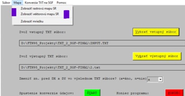
The menu option MAPA/ZOBRAZIŤ VEKTOROVÚ MAPU SR (or MAP/DISPLAY SK VECTOR MAP - between 2 violet bars) displays slovakian vector map (border lines) along with the grid points as can be seen below:

Picture 2 - basic (default) view of the state borders + grid [url=https://postimg.cc/FfkbcrSW]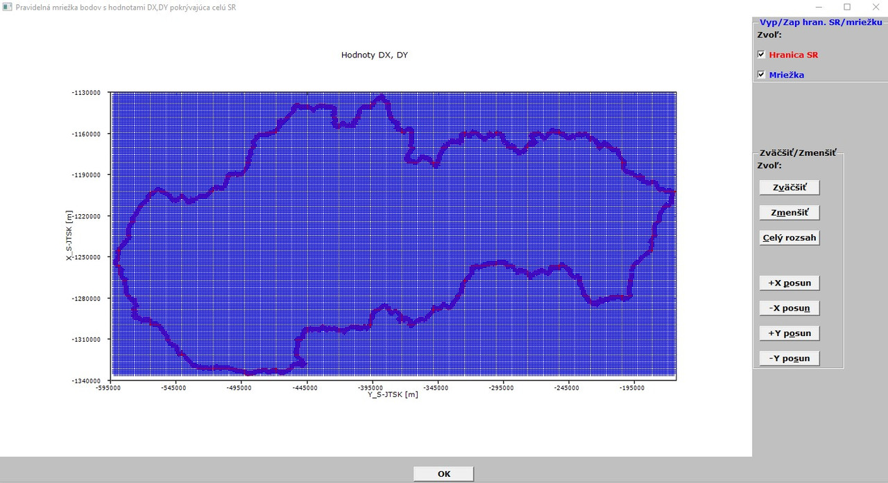

Picture 3 illustrates some pan and zoom in: [url=https://postimg.cc/2VHX75qr]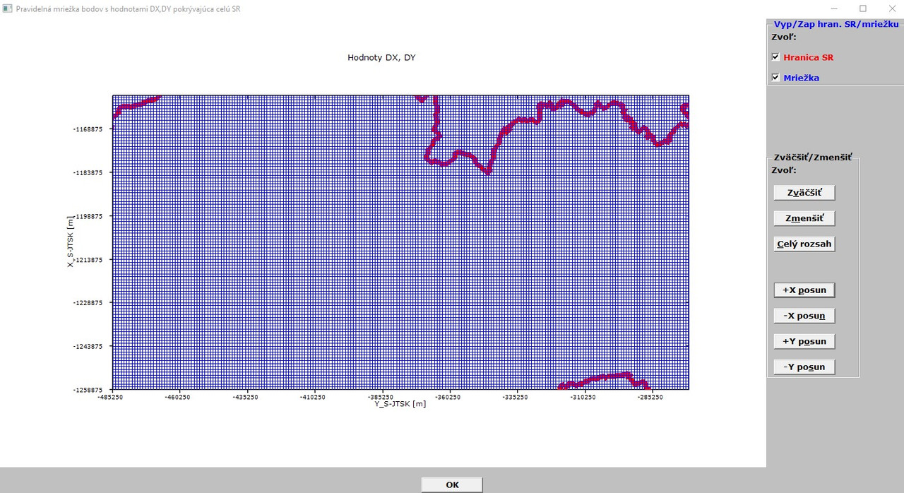

Here is still some problematic point - with the menu option MAP/DISPLAY SK VECTOR MAP (see pictures above), when I click on zoom in/out, move in X/Y directions, zoom to extents - it takes some time (around 8-12 sec) to complete the selected action and sometime the program does not respond for a while (2-3 sec). I know, with this option I have around 135000 points to draw/redraw.

Then, in the menu under MAP option is the third item called ZOBRAZIŤ MRIEŽKU (DISPLAY GRID ONLY).

In the picture below is the default view of the grid (87000+ points to draw/redraw):

](https://postimages.org/) [url=https://postimg.cc/fJ3g5NYd]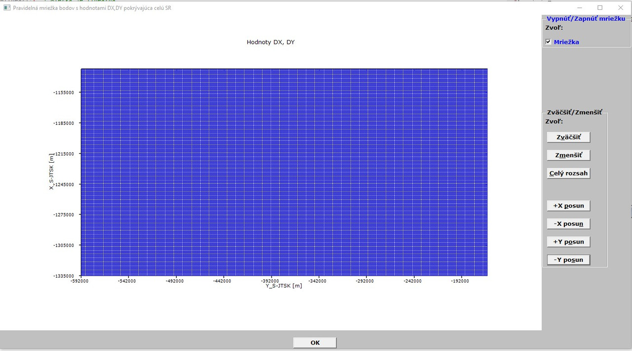 ](https://postimages.org/)

Here, the program reacts little bit quicker (87000+ points only and only rarely does not respond for about 2 sec.

Next picture demonstrates some zooming and pan of grid points only:

[url=https://postimg.cc/mc8xzWv5]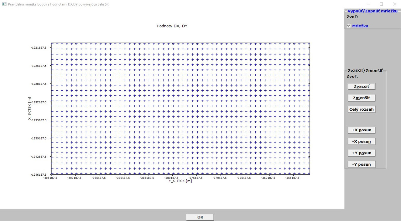

This picture is quite nice and here comes my last dream (of coarse, last dream in conjuction with this program, otherwise I have still many dreams 😄 ).

Namely, I would like to achieve such level of graphics view in the case of grid points that when I will hover with mouse cursor over a grid point, it should display in a small, bordered rectangular area its DX,DY variations.

All grid points have their DX,DY variations and both DX and DY arrays are read in by the program to its memory. Just - how to achieve this. In other softwares points have so-called attributes which can be seen with them in an information window. The DX, DY arrays (although - in reality - they are used for interpolations such as linerar, quadratic, biquadratic) could be displayed in this case as attributes of the grid nodes.

Is here (in FTN95) an attribute function which could help to realize the goal and to assign the DX, DY variations to the corresponding grid node in a small box (similar like bubble help, %bh)?

I could let to create in a DO loop the %bh strings of DX,DY values (87000+ %bh strings), but it sounds crazy and probably unrealistic.

It could be easily assigned, since I read in all 87000+ points along with their DX, DY values.

Thanks in advance for your possible comments!

It may be possible to do something with %pl[full_mouse_input] together with %th[ms_style] and calls to SET_TOOLTIP_TEXT@. Note that %th can be switched on and off and has a delay that can be preset. But it looks like the routine is not documented so I will have to look into that. Here is a brief outline.

SUBROUTINE SET_TOOLTIP_TEXT@(HWND, TEXT) INTEGER(7) HWND CHARACTER*(*) TEXT

HWND is the Windows HANDLE of the control obtain from %lc.

p.s. SET_TOOLTIP_TEXT@ is not working as I expect it to so this post may be premature.

p.p.s. My code now works. See sample in https://forums.silverfrost.com/Forum/Topic/3753.

Martin,

Good to see you are making progress. The code which confused you was for the case where the pixel length of the X and Y axis were to be the same.

One possible way forward, is outlined in the code below. Basically each time the %pl display is refreshed a copy of this is transferred to an internal graphics region. When a mouse move occurs, its coordinates are detected and written to the %pl region using the %gr graphics primitive DRAW_CHARACTERS@. This would quickly fill the screen with text, hence the reason for the stored image which is copied across back to the %pl region immediately before any text is written to the screen.

The values returned by minval and maxval in the %pl call back will already be defined elsewhere in your code.

PS Paul's suggested approach of using %th will be less memory intensive and will also look better with %th[ms_style].

Ken