New sugestion(s) for %PL - (first - an initial question)

Thanks Ken for your important remarks!

However, at this moment I have something wrong somewhere in the code of one (or more?) of the three callbacks dealing with the graphics.

Their full code can be seen/downloaded here: https://www.dropbox.com/s/ben76ov4n02ivs0/PL%2BCB.f95?dl=0

What I am getting now is this:

A short 10s video can be seen here: https://www.dropbox.com/s/k12axnjebx21bzf/jpg_problem.mp4?dl=0

So, the facts are as follows:

1. I need the JPG to be displayed (stretched) ONLY between X,Y axes, not over the whole graph. I have differences between source and destination widths and heights.

I tried it to adjust tentatively in a few iteration by specifying the offset of the image - but I achieve practically nothing, moreover - I do not want to do it manually (to find the values of offset by manually and iteratively trying by typing in their estimated values, since this will always be different from one jpg to the another one). So, in this particular case I would need to shorten (to squeeze) the image both in north-south and east-west direction to get it between X,Y axes and I was unable to find how (I would also need to specify an offset from right bottom corner).

2. As can be seen in the short video, when I load in the raster onto the graph and when I move with mouse (placed outside graph) back over the graph, the image automatically disappears although I used the COPY_GRAPHICS_REGION@ from the buffer on the graph (the ID of the graph is variable handle_pl_OK and equals 0) also in the condition:

IF (cb_reason .eq. 'MOUSE_MOVE' ) THEN

which is in the PL_CB function called within %PL.

Looking only at your graphic above, I suspect that in your call to COPY_GRAPHICS_REGION@

Syntax

INTEGER FUNCTION COPY_GRAPHICS_REGION@(

• DEST_GR, DX, DY, DWIDTH, DHEIGHT,
• SRC_GR, SX, SY, SWIDTH, SHEIGHT, COPY_MODE ) INTEGER DEST_GR, DX, DY, DWIDTH, DHEIGHT,
• SRC_GR, SX, SY, SWIDTH, SHEIGHT, COPY_MODE

you need to subtract the width of the right %pl margin from the present value of DWIDTH, and the height of the bottom %pl margin from the present value of DHEIGHT.

DWIDTH should equal the width X of the %pl graphics region minus the sum of the widths of the left and right margins.

DHEIGHT should equal the depth Y of the %pl graphics region minus the sum of the heights of the top and bottom margins.

X,Y are defined in the %pl call

i= winio@('%pl&',Npoints,X,Y)

DX should equal the width of the left margin.

DY should equal the height of the top margin.

If you have not explicitly specified the margins, use the %pl[margin] option.

[margin=d] Specifies the margin value in pixels for all margins.

[margin=(d,d,d,d)] Specifies values in pixels for the left, top, right and bottom margins.

module demo_margin
use clrwin
implicit none
integer, parameter :: dp=kind(1.d0)
integer, parameter :: mtop = 20, mbottom=300, mleft=300, mright=30
integer, parameter :: npoints = 20
real(kind=dp) :: x(1:npoints),y(1:npoints) 
contains

integer function draw_pl()
integer i, iw
character(len=126) pl_str
  do i = 1, npoints,1
    x(i) = i-1
    y(i) = (i-1)*(i-1)
  end do
  iw = winio@('%mn[Exit]&','exit')
  call winop@('%pl[native,x_array,independent,frame,gridlines]')
  write(pl_str,'('%pl[margin=(',I3,',',I3,',',I3,',',I3,')]')') mleft, mtop, mright, mbottom
  call winop@(pl_str)
  iw = winio@('%pl&',1000,800,npoints,x,y)
  iw = winio@(' ')
  draw_pl =1
end function draw_pl
end module demo_margin

program main
use demo_margin
implicit none
integer i
i = draw_pl()
end program main

John,

Only in the sense that it's sufficiently long to avoid character buffer errors for something like:

'%pl[x_min=-1000.0,x_max=+1000,dx=100,x_sigfigs=2,y_min=-1000.0,y_max=+1000,dy=100,y_sigfigs=2]'

Thanks Ken!

I read the section regarding the COPY_GRAPHICS_REGION@ many times in the on-line manual (which also you pasted in your previous post), but due to its vague formulation I did not understand it as a whole, since I did not know what is the real meaning of DX,DY and SX,SY values. Now, thanks to your explanation I know that he values DX,DY,SX,SY represent margins.

Nevertheless, I still have couple of questions. Please – have a look at the picture below (outlined a pixel coordinate system):

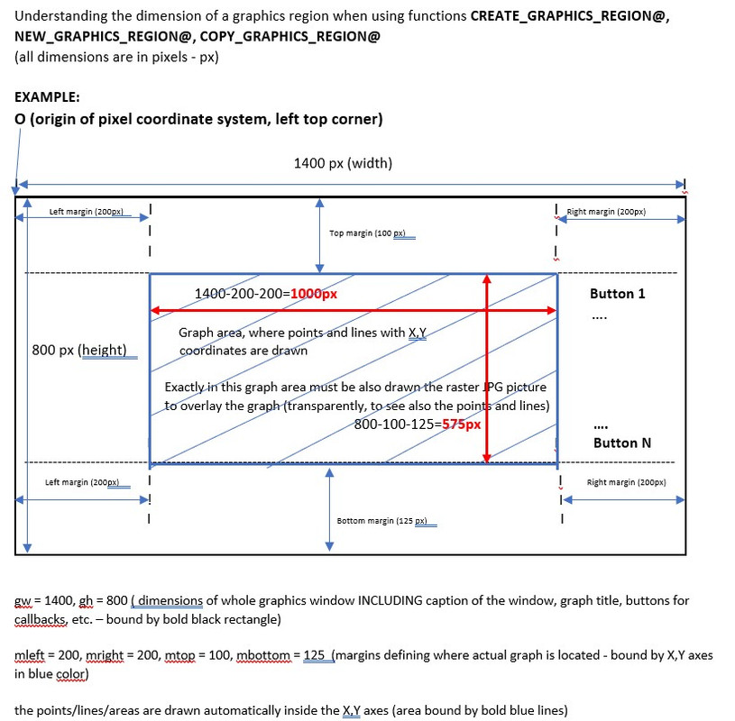
If my understanding (imagination) of a pixel coordinate system pictured above is correct (if not, correct me) the questions are:

A) I defined the whole window area (DW,DH dimensions: 1400x800) to accommodate all texts, buttons, titles, caption, graphs but with NO margin option for the %PL (I did not use the option margin at all). The graph itself, where points and lines are drawn, was automatically created by %PL and bound by X,Y axes. This graph is smaller than 1400x800 window.

**How can I automatically (by program or an option in %PL) detect the pixel coordinates of at least one corner of the graph (say – top left) bound by X,Y axes, where the input data (points) are drawn? **

The procedure with GUESSING the offsets is not usable.

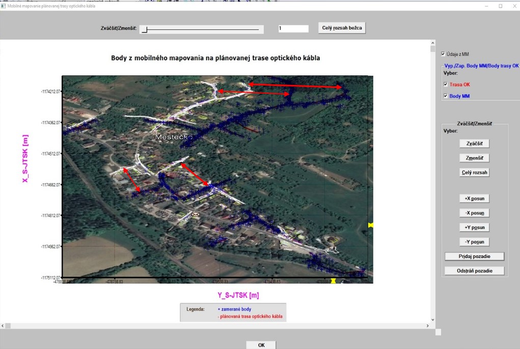
B) When I loaded in the raster jpg image, it was placed within whole white area of the graph (overlaying graph title, X,Y captions and legend). This was – of coarse – not wanted, so I started to try to lower the image dimensions. Unfortunately, I did it manually, tentatively and in few iterations (I started to use the DX, DY values (margins) with 120, 80 – it did not fit, then I used 150, 90, it did not fit and finally – I guessed!!! the correct DX, DY values (200,200), where the top left corner of the vector graphs coincided with top-left corner of the loaded raster image. But this was all, no other dimension coincided, so I posted my questions in my previous post. Based on your answer, I used the MARGIN option for %PL and the result can be seen below:

I used the code (for adjusting raster image to vector graph):

i = COPY_GRAPHICS_REGION@(handle_pl_OK, 200, 100, gw-mleft-mright, gh-mtop-mbottom,  &
                             1001,  0, 0, WIDTH_RASTER, HEIGHT_RASTER, 8913094)

It nearly fits, although not 100% (see two yellow lines in the picture to the bottom right). I could lower it in both directions by value 10 (it would then fit quite good) but then there remain 2 black strips (horizontally and vertically). The question is:

Why – when using GW-MLEFT-MRIGHT and GH-MTOP-MBOTTOM – the image does not coincide exactly to the graph within X,Y bounds?

C) Moreover, although the image was created by me a few months ago, at that time with no intention to use it for such purposes like now, you can see in the picture above (see red lines with arrows) very big displacement of the data when comparing them to the image background). I can investigate how could I create the IMAGE as a raster with no association to real geodetic coordinates in my mobile mapping processing software (where all is treated exclusively and ONLY in real geodetic coordinates and in real geodetic coordinate system), however – I am afraid that this way to overlay the vector data (with real geodetic coordinates) in the graph with an un-georeferenced image (with no coordinate association) is the way to nowhere, impassable and closed.

Nevertheless, it would be great to introduce an internal function like GET_DATA_SCALE@ which would output the graph scale (which scale in the graph is used for the drawn data by %PL. All maps have a scale like: 1:500, 1:1000, 1:10000, … Or to have a possibility to specify a particular scale info to %PL (I do not mean current scale options for %PL like SCALE=LINEAR,… I mean to tell %PL to draw all input data in linear scale – let say – 1:1000, it means SCALE=1000 or SCALE = 500, …).

still last sentence of my previous post:

I do not mean current scale options for %PL like SCALE=LINEAR,… I mean to tell %PL to draw all input data in linear scale – let say – 1:1000, it means SCALE=1000 or SCALE = 500, …).

Works very well in this example:

https://www.dropbox.com/sh/n3x2o37tzlpb14u/AAAwtVLFlno5gLvN3a9f-SI6a?dl=0

Re item C)

Surely you know the physical coordinates corresponding to the top left and bottom right corners of your image, and GET_DIB_SIZE@ gives you the dimensions of the image in pixels.

So for the horizontal direction the physical coordinates of the image range from xmin to xmax, and the pixel coordinates of the image range from 1 to width (or pmax) returned by GET_DIB_SIZE@.

For the physical range [xmin,xmax] and the pixel range [1,pmax], then a value x in the range [xmin,xmax] is linearly mapped to a value p in the range [1,pmax] (using real arithmetc) as

p = 1 + (x-xmin)*(pmax-1)/(xmax - xmin)

Same for the vertical direction.

The top left and bottom right pixel coordinates of the %pl frame can be calculated from the %pl graphics width, height, and margins.

The corresponding physical coordinates can be determined from GET_PLOT_DATA@.

Using these physical coodinates and the linear mapping, you can calculate SX, SY, SWIDTH, SHEIGHT for COPY_GRAPHICS_REGION@ for any x and y ranges displayed by %pl, such that the different coordinate systems are correctly aligned.

Unfortunately, I cannot comment on the correction of planar (stretch) distortion in your image.

**PS The required mathematics to undistort photographs taken of a flat piece of land photographed from an angle are clearly described here ** http://paulbourke.net/geometry/transformationprojection/

Many thanks for your kind help, Ken!

Now, it is clear and understandable what means a pixel coordinate system and how it is associated with real geodetic coordinates in the graph. It is pity that such essential information is not available in the on-line help (at least – I did not find it there).

Based on your explanation I added automatic computation of graph´s scale, which is written next to the graph as can be seen below (scale is an important and essential information for any surveyor when dealing with graphs/maps):

I plan to add to the graph above in the future also some statistical data for lines (like total line length, line length of each segment and maybe more – simply properties of each map´s object. I hope, I will be able to do it, since it requires quite extensive coding and the use of drawing functions of FTN95. With respect to the scale in the graph above I have two simple questions:

1. As can be seen in the picture above, the computed scale is exact scale based on pixel and meter conversion (1px = 0.0002645833m) between two pairs of identical points having both pixel and real geodetic coordinates. However, I would like to round it (since the scale like the one in the graph – 1:33927 is very unusual). Is there an intrinsic function in FTN95 (I do NOT mean ANINT/CEILING/FLOOR functions since it seems to me that they do not provide what I exactly want) which would round the number provided as argument to the whole tens or hundreds? (I mean – for example – to round the scale 1:33927 to 1:33900 or 1:34000).

Although, it would be a little bit deceptive, it looks much better.

2. I would also like to import to the graph a north sign (north arrow) which points to the north. Should I use the same functions (GET_DIB_SIZE@ and IMPORT_FILE_IMAGE@) like in the case of JPG import?

Regarding your answer to the item C and the link you provided: Thanks. The datum transformations and different map projections was/is my professional job. This was main topic of my dissertation of which practical result was a software called DatTra – Datum Transformation which computes 3D transformations between global geocentric coordinate systems like WGS-84 (World Geodetic System 1984) and/or ETRF-89 (European Terrestrial Reference Frame 1989) and our local coordinate systems used in Slovakia (System of unified cadastral network – S-JTSK, based on local Bessel´s ellipsoid and Krovak´s projection and a former military coordinate system S-42 (based on Krasovsky´s ellipsoid and Gauss-Kruger projection, which is similar to UTM – Universal Transversal Mercator projection) and vice-versa. In the past, we had the DatTra package (of which I am main co-author) as standalone utility, but now – we also have it in DLL version which can be built-in in any GIS software package. In fact, it is also built-in in such packages like ESRI ArcGIS or Q-GIS. They have a default transformation also for Slovakia, nevertheless it is not precise enough, so some customers in Slovakia with the highest requirements with respect to accuracy selected to built-in our DLL functionality.

With respect to the distortion of the raster JPG image overlayed in the graph of points/lines: I am afraid that it cannot be fully aligned, since the raster JPG is pure image with no coordinate association (therefore I suggested to have an option in %PL to load in a geo-referenced image). Maybe it can be reduced with much effort.

Martin,

This may help, but the question of rounding numbers (particularly negative numbers) opens a 'can of worms'. This function round_n10 rounds to a power of 10 symmetrically about zero. Where the input data would cause an integer overflow, the returned number is simply returned unrounded.

winapp
program rounding
implicit none
integer, parameter :: dp=kind(1.d0)
real(dp) x
integer i, p
x = 1234567.89123d0
print*, 'Positive x ', x
print*, 'Rounded to different powers of 10'
do p = -6, 6, 1
  print*, p, round_n10( x, p), int(round_n10( x, p))
end do

x = -x
print*
print*, 'Negative x ', x
print*, 'Rounded to different powers of 10'
do p = -6, 6, 1
  print*, p, round_n10( x, p), int(round_n10( x, p))
end do

print*
p = 2
do i = -52,-48, 1
  x = i
  print*, 'x =', x, 'p = ', p, round_n10( x, p), int(round_n10( x, p))
end do

print*
p = 2
do i = 48,52, 1
  x = i
  print*, 'x =', x, 'p = ', p, round_n10( x, p), int(round_n10( x, p))
end do

contains

real(dp) function round_n10(in,p)
real(dp),  intent(in)  :: in     ! Number to be rounded
integer, intent(in)    :: p      ! Power of ten to which number is to be rounded
real(dp) a, b, e, t
     e = (10.d0**(p))
     if (in .gt. 0.d0 .or. in .lt. 0.d0) then
       t = in/e
     else
       round_n10 = 0.d0
       return
     end if
     if (abs(t) .ge. huge(1)) then  ! Integer overflow case, no rounding applied
       round_n10 = in
       return
     end if
     a = nint(t)*e
     b = -a + e
     if (in .gt. 0.d0) b =  a + e
     round_n10 = a
     if ( in - a .gt. b ) round_n10 = b
end function round_n10

end program rounding

Or more simply:-

real*8 :: x = 33927.d0
print*, x
print*
print*, 1.d0    * NINT(x)
print*, 10.d0   * NINT(x / 10.d0  )
print*, 100.d0  * NINT(x / 100.d0 )
print*, 1000.d0 * NINT(x / 1000.d0)
end 

Great Ken!

The one-line code for rounding is brilliant (to paraphrase a classic: all brilliant ideas and their beauty ground in their simplicity). In the meantime, I added the logo for N/S/E/W directions as can be seen in the picture below (the letters in the logo are in slovakian: S=sever/north, J=juh/south, V=východ/east, Z=západ/west). As can also be seen in the picture, I was able to adjust the JPG image exactly between the axes (what I also wanted). However, this was achieved (again) by experimenting only.

I use the code for adjusting JPG image in the graph (after its import using IMPORT_FILE_IMAGE@) as follows:

i = COPY_GRAPHICS_REGION@(handle_pl_OK, mright, mtop, gw-mleft-mright, gh-mtop-mbottom,  &
  1001,  0, 0, WIDTH_RASTER, HEIGHT_RASTER, 8913094)

where mright, mtop, mleft, mbottom are values for graph´s margins in all directions defined as parameters in declarations. The same is valid also for GW (graph width) and GH (graph height). WIDTH_RASTER, HEIGHT_RASTER are values of JPG width and height provided by calling the function GET_DIB_SIZE@ (in my case WIDTH_RASTER=612 and HEIGHT_RASTER=575). However, the code above never fitted the JPG exactly between X,Y axes. The JPG was always overlapping behind both axes a little bit (a picture in one of my previous post demonstrates it). I believe that the reason for it is that JPG was adjusted automatically taking also into account the number values indicated below tick marks on both axes as something which belongs to the graph area.

So, I manually adjusted the JPG image by using values -5,-5, then -10, -10 instead of 0,0 in the code above. It brought some improvements, but not 100%.

Therefore, I tried to experiment with the code:

i = IMPORT_FILE_IMAGE@( 'orthophoto_and_geo_surveying.jpg' , -10, -15 )

The code above with the offsets of -10, -15 works very well (see the picture above). Since the values X (in my case -10) and Y (in my case -15) represent the pixel offsets into the %PL graphics region – I would like to know a general rule – how to determine their right values automatically by the program before copying it to a selected %PL graphic region.

I tried some combination with the values I use for dw (1400),dh (800), mright (200), mleft (200), mtop (100), mbottom (125), WIDTH_RASTER (JPG) = 612 and HEIGHT_RASTER(JPG) = 575 to get the pixel offsets X,Y for IMPORT_FILE_IMAGE@, but I got never the values -10 and -15, which are the right values for this purpose.

Martin,

Why is the second argument passed to COPY_GRAPHICS_REGION@ the variable MRIGHT?

Suggest you print out all the relevant variables so that you can do a manual check.

Also are you getting mixed up between gw, gh, and dw, dh ?

Is there a %pv in your code before the %pl? That might be causing problems since the graphics width and height of the %pl will change when the user resizes the window - I can see you have used %ww which permits this.

Ken,

see my picture of how I understand the pixel coordinate system on the display in my post of Mon Mar 22, 2021 11:24 am in this conversation.

So, the WHOLE window area (it means whole size of the windows, where all these things are displayed) has the following dimensions:

width (gw) = 1400, height (gh) = 800

This size 1400x800 of the whole window includes all (caption of the window, graph itself and buttons to the right and also the OK button at the bottom).

The graph itself (where lines, points and raster JPG image are drawn and displayed) has the dimension of 1000x 575 since I used the margins mright=200, mleft=200, mtop=100 and mbottom=125 (so 1400-200-200=1000 and 800-100-125=575).

As I understand it, the origin of my drawing surface (area of 1000x575) has its pixel coordinates at the values MLEFT, MTOP. And YES, formally it is an error to use MRIGHT (my mistake - thanks for revealing it, I already corrected it to MLEFT, but in this specific case, it caused no harm due to the fact that MLEFT=MRIGHT=200). Therefore I used the variable MLEFT in the COPY_GRAPHICS_REGION@ as one of its offset values to be able to paste the top left corner of the JPG raster exactly on the top left corner of may graph area (on its origin).

Maybe I should somehow compute the SX, SY values, since in the copy function I use for them both ZERO values.

The dh is my typing error and is - in fact - gh (I do not use the dh variable in my program at all). Although I use %ww, I have NO use of %pv within the whole program.

I will check all above mentioned variables once again by printing them out to visually confront their values - as you suggested.[/b]

OK, you have told me the same thing twice, and I thought it was incorrect the first time.

If width (gw) = 1400, height (gh) = 800 are the values used to define the %pl region, then this is not the size of the whole window.

These sizes define the size of the rectangular graphics area into which the %pl graph including its margins are drawn.

The buttons on the RHS and the OK button are not in the graphics region. They are in the ClearWin+ window, as is the %pl graphics region which has the dimensions specified in the winio@ call which sets up the %pl.

Here is a simple example, which draws two graphs sequentially. The size of the %pl graphics region is the same in each case, but the overall window size differs.

      WINAPP 
      USE clrwin 
      INTEGER N,im,gw,gh
      PARAMETER(N=10,gw=600,gh=300)
      REAL*8 x(N),y(N)
      DO i=1,N
        x(i)=0.1d0*(i-1)
        y(i)=x(i)*x(i)
      ENDDO
      i=winio@('%ca[Quadratic]&')
      i=winio@('%bg[blue]&')
      i=winio@('%`bg[white]&')
      CALL winop@('%pl[title=Graph,width=2,y_max=0.9,x_array,link=curves,symbol=9,colour=red,pen_style=2,framed]')
      i=winio@('%pl&',gw,gh,N,x,y)
      i=winio@('%sf%ff%nl%cn%tt[OK]')
      i=winio@('%ca[Quadratic]&')
      i=winio@('%bg[blue]&')
      i=winio@('%`bg[white]&')
      CALL winop@('%pl[title=Graph,width=2,y_max=0.9,x_array,link=curves,symbol=9,colour=red,pen_style=2,framed]')
      i=winio@('%pl&',gw,gh,N,x,y)
      i=winio@('%ta%ta%sf%tt[OK]')
      END

Thanks Ken for your correction of my wrong imagination! I will try to find out how to compute in the program the offsets for imported JPG raster image (IMPORT_FILE_IMAGE@ offsets) BEFORE pasting it on the graph to coincide exactly with the axes.

Now, I added some statistics to the graph (in yellow rectangle). All numbers there are variables extracted from input data:

I would like to use different colors for the numbers (red for all) in the statistics (8.5 km is length of the route, 20 means different sections of the route, 2098 means number of surveyed points during mapping of the route and 57.12m is the maximum height difference between two points).

So the text would be black as it is now and the numbers (variables) would be in red.

I use the following code to write a string (for SCALE as example):

WRITE (output_string(5),fmt(5)) 'Mierka=1:', I_MIERKA
CALL draw_characters@(output_string(5),gw-190,mtop+130,rgb@(51,25,0))

How to achieve that the text will be in black (as is now) and the number would be in red when the function DRAW_CHARACTERS@ requires as its 4th argument one color only and the text and the value (variable for scale) are both written to one output string (output_string(5)) ? (I do not want to use 2 lines for it - one line for text in black and one line for the variable scale. This I can do with two colors. I want to have in one line two different colors).

Thanks in advance for some inspiration!

Martin,

Split each of output strings into two strings, one with the description and one with the number values.

The first is written using draw_characters@(description(i),x,y,rgb@(0,0,0))

The second is draw_characters@(number(i),x+offset,y,rgb@(255,0,0))

In each case the x,y will be the current coordinates you are using, and offset chosen to align all the numerical values.

Note that the pixel length (and height) of x(i) is returned by GET_TEXT_SIZE@, but you need to use TRIM since the length returned by this includes trailing blank characters.

call GET_TEXT_SIZE@( trim(adjustl(txt))//achar(0),tw,th )

This could be used in a simple DO LOOP to determine automatically the length of the longest description string and this plus and extra few pixels determines your offset (and avoids some alignment problems when you change the descriptions at a later date [however the margin may be too small]).

Re: IMPORT_FILE_IMAGE@ offsets, since you don't have a %pv, I cannot see a reason why this is necessary. You might want to try a) importing a different file (size in pixels), and/or changing the %pl graphics size. The results, what ever they are may help pinpoint where the problem lies. Are gw and gh, as well as your margins truly global values, or do you have local declarations with the same name in some of your routines? For example, consider the chaos this example could result in:

module t
implicit none
integer, parameter :: gw = 100
contains
  integer function run1()
  print*, 'gw = ',gw
  run1=1
  end function run1

  integer function run2()
  integer gw     ! local declaration
  gw = 2000
  print*, 'gw = ',gw
  run2=1
  end function run2
end module t

program main
use t
i=run1()
i=run2()
i=run1()
end program main

Thanks Ken!

I will do it as you suggested.

After your explaining what are the graph´s dimensions (I mixed it with window dimensions) I made some additional steps and the graph/map looks like this:

Now, the graph/map above contain all essential (from geodetical point of view) information to properly interpret the data which it contains (scale, info about horizontal and vertical coordinate system, north arrow, number of objects). It is intuitive that the text in red in the statistic relates to the red objects in the graph (red lines), the text in blue relates to the blue objects (blue points). Nevertheless, I will improve it as you suggested (text in black and numbers in red/blue), since sometimes too many colors can be extravagant.

Regarding the importing of JPG raster image to the graph - have a look please to my code below:

...
iw = CREATE_GRAPHICS_REGION@( 1001, WIDTH_RASTER, HEIGHT_RASTER)
          i = IMPORT_FILE_IMAGE@( 'orthophoto_and_geo_surveying.jpg' , -10, -15 )
i = COPY_GRAPHICS_REGION@(handle_pl_OK, mleft, mtop, gw-mleft-mright, gh-mtop-mbottom,  &
                             1001,  0, 0, WIDTH_RASTER, HEIGHT_RASTER, 8913094) !! 13369376)!! 8913094) 

Note that in the COPY_GRAPHICS_REGION@ I use ZERO offset, but in the IMPORT_FILE_IMAGE@ I use the offsets -10 and -15.

Using the code above, JPG is correctly pasted between X,Y axes (no overlapping of axis and tick mark values). When I used them as ZERO values for IMPORT_FILE_IMAGE@ and -10,-15 for COPY_GRAPHICS_REGION@, the image overlaps BOTH the axes AND the tick mark values below axes exactly to their bottom (the same when I use ZERO values for both commands).

I am confused from it and don´t know how to interpret it (I already said earlier in one of my previous post that it seems to me that IMPORT_FILE_IMAGE@ command may interpret where to paste it also the tick mark numbers as whole graphics region and therefore it stretches the image also over them).

So, the question remains - how could be determined the right offset for the IMPORT_FILE_IMAGE@ in advance BEFORE pasting it to the graph (not by experimenting by trying to manually input some estimated values).

The above mentioned variants of offsets and their impact on the graph are demonstrated here:

https://www.dropbox.com/s/kptg0wxd432g4qn/offsets.pdf?dl=0

Add the following immediately after you call to COPY_GRAPHICS_REGION@

call set_line_width@(2)
call draw_rectangle@(mleft, mtop, gw-mright, gh-mbottom, rgb@(255,0,0))
call set_line_width@(1)

If this rectangle aligns with the %pl frame, then you eliminate the destination graphics region as the source of the problem. However I think you may well find that the lower right hand corner is offset by 10 pixels to the right and 15 down.

Here is how the graph looksafter implementing your test code with rectangle:

It seems to me that my assumption was correct and it was that the destination graphics region (its dimensions) also includes the number below tick marks (its bottom or base of the numbers) - not only axes as such as can be seen in the picture above. Probably this is also the reason why JPG raster image is stretched in such way that it also overlaps axes and the numbers below tick marks and ends exactly at the base of the numbers.

So, the question is how to automatically compute these values to eliminate it.

Important note:

I moved the following code from a call-back, which loads in the JPG raster image to the beginning of my plot function which uses %PL:

CALL GET_DIB_SIZE@( 'orthophoto_and_geo_surveying.jpg', WIDTH_RASTER, HEIGHT_RASTER, NBBP,ERCODE )
iw = CREATE_GRAPHICS_REGION@( 1001, WIDTH_RASTER, HEIGHT_RASTER)
i = IMPORT_FILE_IMAGE@( 'orthophoto_and_geo_surveying.jpg' , 0, 0 )
iw = CREATE_GRAPHICS_REGION@(handle_internal_gr,gw,gh)

Earlier, the code above was part of the call-back assigned to the button for loading in JPG ratsre image:

INTEGER FUNCTION pridaj_raster ()
IMPLICIT NONE

   
 !!  CALL GET_DIB_SIZE@( 'orthophoto_and_geo_surveying.jpg', WIDTH_RASTER, HEIGHT_RASTER, NBBP,ERCODE )  
 !!  i = NEW_GRAPHICS_REGION@( 1001, WIDTH_RASTER, HEIGHT_RASTER, rgb@(0,0,0))
 !!  i = IMPORT_FILE_IMAGE@( 'orthophoto_and_geo_surveying.jpg' , -10, -15 )
 i = COPY_GRAPHICS_REGION@(handle_pl_OK, mleft, mtop, gw-mleft-mright, gh-mtop-mbottom,  &
                             1001, 0, 0, WIDTH_RASTER, HEIGHT_RASTER, 8913094) !! 13369376)!! 8913094) 
   pridaj_raster = 2
END FUNCTION pridaj_raster

Now, even when I use the offset values -10,-15 in the IMPORT_FILE_IMAGE@, although it does align with axes, but a vertical and horizontal black strip remains in the graph exactly in the space which overlaps the axes and tick mark numbers. So, I use 0,0 values.

John,

After moving the code as described above and using offsets -10, -15 the result is:

I meant the black strip in vertical and horizontal direction as can be seen in the picture above. So, I have to use 0,0 offset (then no black strip appears, but overlapping remains with raster image exactly in the area, where black strips are.

The reason for black strip is clear - COPY_MODE 8913094 since it copies as follows: The colors of the source and destination areas are combined using the Boolean AND operator. And when they NOT EXACTLY FIT (are NOT exactly aligned) then the result is as in my picture.